HANDY - Basics

Table of Contents

• Home
• Install
• Basics
• Regions and ranges
• Points
• Radial velocity correction
• Grids

Basic workflow

1. Load spectrum for analysis
2. Compute theoretical spectrum and correct processed spectrum for radial velocity (see more: Radial velocity correction)
3. Define or load region/ranges and special Points (see more: Regions and ranges, Points)
4. Establish some initial parameters by visual comparizon with spectrum from grid (see more: Grids)
5. Save normed spectrum and continuum file. Decide if you want to save radial velocity corrected spectrum or not.
6. Load new spectrum and continue…

Menu

• Open
  • Open spectrum - loading spectrum for processing. Works with ASCII and FITS files. HANDY does not use any information from header part. Defaults for ASCII format are (this properties can be modified globally in spectrum.py file):
    • 1st column - wavelength
    • 2nd column - flux
    • without header
    • ’#’ are the first character in comment lines
    • whitespace delimited
  • Open continuum file - enable user to load predefined file with regions/ranges and special Points definitions (see more: Regions and ranges, Points)
  • Open theoretical spectrum - load some spectrum for comparison, only ASCII format
  • Exit - close the HANDY program
• Save
  • Save normed spectrum - saving normalized spectrum with oryginal wavelengths table, only ASCII format
  • Save normed spectrum VRAD corrected - saving radial velocity corrected normalized spectrum, only ASCII format
  • Save continuum - saving definitions of regions/ranges and special Points
  • Save theoretical spectrum - saving theoretical spectrum, only ASCII format
• Grids
  • here apears names of predefined grids defined in gridsDefinitions.yaml file (see more: Grids)

Plots

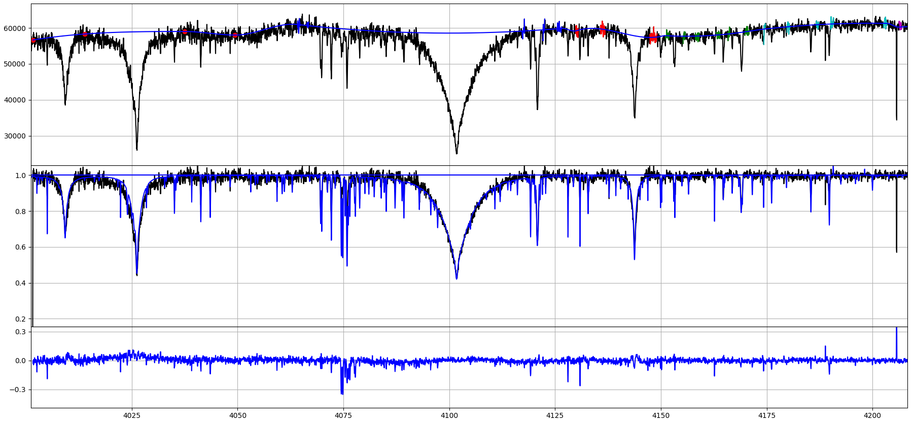
• Top plot
  • Black line - observed spectrum which we are working on
  • Blue line - fitted continuum
  • Red points - special points
  • Short blue/red/green/magenta/cyan/purple parts - each color denotes single region, while each highlighted part called range
• Middle plot
  • Black line - normed observed spectrum which we are working on (spectrum/continuum)
  • Blue line - loaded theoretical spectrum
• Botton plot
  • Blue line - residuals of fit (normed spetrum - theoretical spectrum)

Buttons

• Back - load last regions/ranges (note: does not modify Points)
• Choose region/scroll wheel click - make it possible to change active region by clicking above it
• Create region - next added range will belong to newly created region and become the actve one
• Next spectrum - Not implemented yet
• Add special point - next click on spectrum will add special Point (more here: Points)
• Auto fit special points - automatically normalize all special Points relative to theoretical spectrum
• Normalize - apdate normalization once - usefull when we do not want normalization to update automatically
• Auto update - when clicked after any modification of ranges/Points/uploading continuum, etc. normalization will automatically update
• Radial velocity - open radial velocity correction dialog (note: works only when theoretical spectrum is loaded; more here: Radial velocity correction)
• Adjust order spinbox - changes order of chebyschev polynomial fitted to active region

Grid interface panel

• Clear theoretical spectrum - clears theoretical spectrum from second plot
• Compute theoretical spectrum - interpolate theoretical spectrum of parameters given by sliders values
• Sliders and resolution spinbox - enable user to set parameters of theoretical spectrum

Working with already normed spectrum

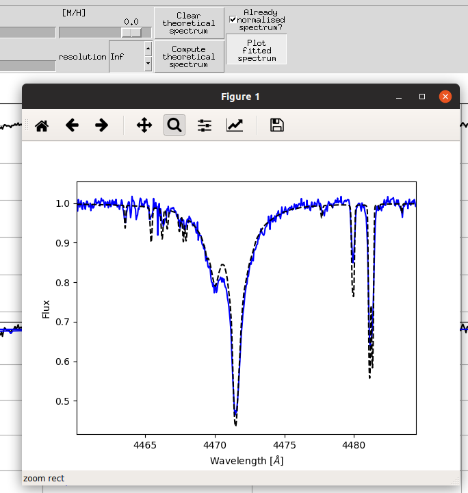
• Checkbox Already normalised spectrum - Use loaded spectrum as normalized spectrum. When checked it is only possible to correct spectrum for radial velocity and do comparison to theoretical spectrum
• Plot fitted spectrum - plots normalized spectrum and model spectrum in x-range taken from main plot, and enable user to save the picture for future inspection